GML Newsletter: Homophily, Heterophily, and Oversmoothing for GNNs
"Birds of a feather flock together"
Hello and welcome to newcomers!
In this email, I will look into recent research that focuses on the performance of GNNs in two opposing settings, homophily and heterophily, and its connection to oversmoothing.
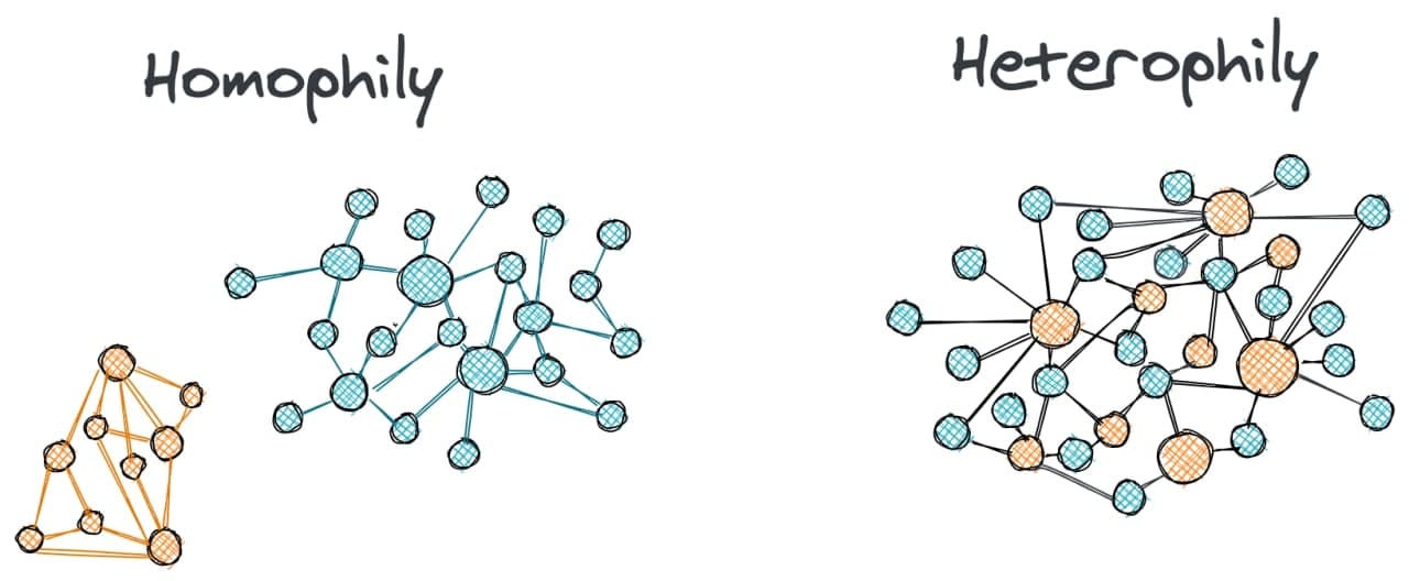
The term homophily in network science means that nodes of the same group or label tend to cluster together. The group here is defined informally and depending on its definition homophily may or may not arise in your network. So, for example, in a social network people that graduated from the same university tend to be connected together and the network is homophilous with respect to the university label.
Opposing homophily is the term heterophily when nodes of different groups tend to be connected, while the connectivity within the groups is sparse. For example, fraudsters in transaction networks are more likely to be connected to accomplices than to other fraudsters. In this case, fraudsters form heterophilic connections with the nodes of accomplices.
One of the popular ways to define homophily in a network is as a fraction of edges that connect nodes with the same label. This ratio h will be 0 when there is heterophily and 1 when there is homophily. In most real applications, graphs have this number somewhere in between, but broadly speaking the graphs with h < 0.5 are called disassortative graphs and with h > 0.5 are assortative graphs.
Why is it interesting? In my opinion, there is a mini paradigm shift in the GNN community that happened over the last year. This shift is associated with increasing evidence that popular message-passing networks such as GCN or GAT that aggregate messages locally do not work well with the disassortative graphs and new insights and architectures have been discovered to make it work. Let’s look at what happened.
How it all started
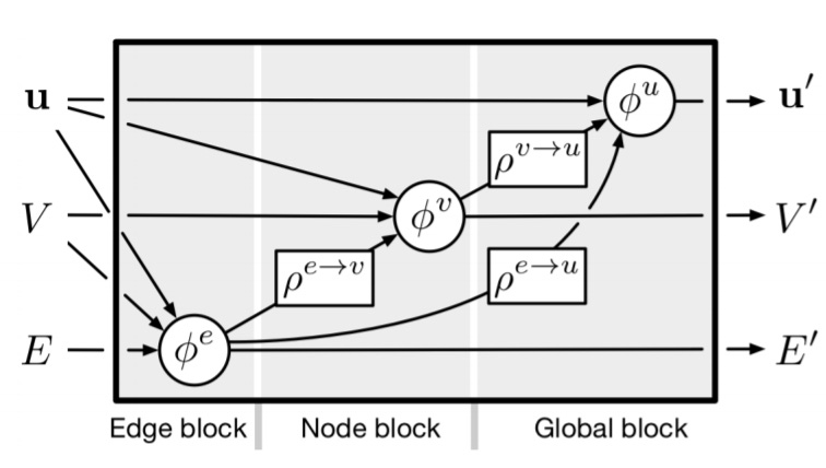
When we think of graph neural nets, arguably the most generic architecture we imagine is the message-passing neural net. This model takes a graph with node and edge features and then synchronously updates these node and edge features using neighborhoods of each node.

This architecture leaves us with many design choices that we have to make before applying it to real graphs. In particular, we need to decide how exactly the model updates the node and edge features, i.e. what functions do we need to apply to the input, how do we define the neighborhood for each node, and how do we aggregate the neighbors.
These choices led to hundreds of architectures, each claiming its SOTA on Cora datasets. For example, one of the first models of this kind, GCN, takes the sum of 1-hop neighbors’ embeddings multiplied by a learnable weight and normalized by the degree.
You can see that the neighborhood is just 1-hop neighbors, the aggregation function is the summation, and the transformation functions are linear projections into latent space.
And these models indeed show improvement on some datasets. For example, if you compare GCN with node2vec or MLP on Cora dataset you will get 10-30% increase in accuracy metric. That was a huge deal and sparked a lot of interest in studying graph neural nets. There were just two issues with that.
Back to the modern days
The first issue is a rather reputational one. With all the hype that deep learning has graph researchers also want to brag that we have deep graph neural nets that solve important real-world problems. But if you start increasing the number of layers in GCN, then surprisingly performance starts going down. Shortly after introducing GCN, Li et al. 2018 explained that vanilla message-passing nets essentially perform a Laplacian smoothing that may mix features of vertices from different clusters and make them indistinguishable. This problem was called oversmoothing and received hundreds of papers that tackle it.
The second problem is a practical one. In parallel, with new SOTAs on Cora datasets, there were other datasets where message-passing GNNs do not outperform simple baselines that sometimes ignore graph structure altogether. More recently Huang et al. 2021 showed that in high-homophily regimes label propagation with 0 parameters is capable to attain the same or better performance than complex GNNs with millions of parameters. What’s going on?
My bet is that we still have not figured out the whole palette of applicability for GNNs, but there are recent results that show that those datasets where traditional message-passing networks do not work well are disassortative graphs, while Cora and co. are all assortative graphs. Moreover, it turned out that oversmoothing and heterophily are deeply linked and it’s possible to design GNNs that are both deep and perform well on the homophily and heterophily settings. Let’s see what happened.
Fixing the problems
A background idea of heterophily is that neighboring nodes can be of different classes and it’s not good for GNN to treat nodes in the neighborhood equally. Some models like GAT have an additional learnable weight per edge, but this weight is positive and rather plays a role of a balance that decides how much of a neighbor we need to put in the aggregation function. Instead, we need to redefine the whole notion of a neighborhood for a GNN, and here is how new architectures do it.
One way was proposed by Pei et al. 2020, where Geom-GCN architecture first embeds nodes in the latent space and then builds a new graph between embedded points. As such the neighborhoods are parameterized and redefined at each step. FAGCN of Bo et al. 2021 in turn takes the approach of GAT to learn the weight on each edge; however, they allow the weight to be negative as well. This can be seen as splitting the neighborhood into two: the positive and negative parts. One limitation of this is that the approach is tailor-made to the input graph and as such the model is transductive.
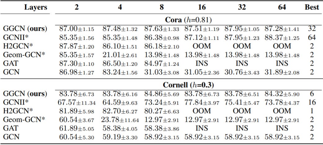
To fix this, Yan et al. 2021 proposed an inductive setting for GNNs that define + and - for each message in a differentiable style in their GGCN model. Moreover, they back up their model design by some theoretical explanation on how oversmoothing and homophily are related. In particular, they show that nodes with high heterophily or nodes with low heterophily and low degree cause oversmoothing problem by moving to the mean embedding of the opposite class. You can see from the image below how the performance of their model does not degrade, going up to 64 layers.

Finally, in addition to redefining the neighborhood per se, some hacks were proposed to change the way models aggregate the nodes. Zhu et al. 2020 offered 3 tricks in the H2GCN model: a concatenation of ego embedding with neighborhood one, using 2-hop neighborhoods, and combining all hidden layers into final representation. Another approach was inspired by ResNet by Chen et al. 2020 who proposed GCNII model that includes two more tricks: using residual connections to the initial representations and adding identity matrix to the weight matrix at each layer. These tricks were known before and could be applied to a wide range of message-passing networks but the authors prove their relevance to solving oversmoothing in disassortative graphs.
These new architectures were evaluated in a wide range of graphs, showing their applicability in heterophily settings. The problem of oversmoothing seems to be solved as well unless there are some other datasets where the proposed architectures degrade performance with more layers. Nonetheless, the global question of when to apply GNNs vs other (non)-graph models remains open.
That’s all for today. If you like the post, make sure to subscribe to my twitter and graph ML channel. If you want to support these newsletters there is a way to do this. See you next time.
Sergey


